``God plays dice with the universe,'' is [Joseph] Ford's answer to Einstein's famous question. ``But they're loaded dice. And the main objective of physics now is to find out by what rules were they loaded and how can we use them for our own ends.'' [8, p.314,]
Chaos brings to mind images of complete randomness, of disorder and anarchy. It is a messy room, a mob rushing down a city street and a swarm of bees. In 1986, at a conference on mathematical chaos held by the Royal Society in London, mathematicians were asked to define the ``chaos'' that had become the buzzword for their hot research area. After much deliberation, they offered the following:
Stochastic behavior occurring in a deterministic system. [22, p.17,]
As definitions go, this one is particularly constipated and quite far from fostering any intuition about the subject. In Stewart's Does God Play Dice?, he claims knowledge of the etymology of stochastic in the statement, ``The Greek word stochastikos means `skillful in aiming' and thus conveys the idea of using the laws of chance for personal benefit.''[22, p.54,]
According to Stewart, stochastic behavior is probabilistic behavior. Probability is that ``other branch'' of mathematics - the one that can't give any specific answers to the outcomes of systems, but can predict how likely a particular outcome is. A single die roll is a probabilistic system: there's a one in six chance that the roll will end with the four face up. We can't predict the outcome of the die roll, but we can assign some numbers to how often certain events will happen.
By placing both stochastic and deterministic in the same definition, the mathematicians have formed a bridge between the two sciences - two sciences that were regarded as mutually exclusive until then. Chaos is the study of deterministic systems that are so sensitive to measurement that their output appears random.
Edward Lorenz found out all of that the hard way. In 1961, he had managed to create a skeleton of a weather system from a handful of differential equations. He kept a continuous simulation running on an extremely primitive computer that would output a day's progress in the simulation every minute as a line of text on a roll of paper. Evidently, the whole system was very successful at producing ``weather-like'' output - nothing ever happened the same way twice, but there was an underlying order that delighted Lorenz and his associates.
...Line by line, the winds and temperatures in Lorenz's printouts seemed to behave in a recognizable earthly way. They matched his cherished intuition about the weather, his sense that it repeated itself, displaying familiar patterns over time, pressure rising and falling, the airstream swinging north and south.[8, p.15,]
What Edward Lorenz had discovered was a chaotic system. Even though a computer had control of the simulation, and certainly possessed the capability to generate random numbers at will, there was nothing random about any portion of the way the simulation was supposed to work. It merely followed the laws of calculus as set down by Sir Isaac Newton himself and outputted a day's worth of virtual weather at the end of each minute. Lorenz's initial brush with chaos is described best by James Gleick's own words, from Chaos
One day in the winter of 1961, wanting to examine one sequence at greater length, Lorenz took a shortcut. Instead of starting the whole run over, he started midway through. To give the machine its initial conditions, he typed the numbers straight from the earlier printout. Then he walked down the hall to get away from the noise and drink a cup of coffee. When he returned an hour later, he saw something unexpected, something that planted a seed for a new science.This new run should have exactly duplicated the old. Lorenz had copied the numbers into the machine himself. The program had not changed. Yet as he stared at the new printout, Lorenz saw his weather diverging so rapidly from the pattern of the last run that, within just a few months, all resemblance had disappeared. He looked at one set of numbers, then back at the other. He might as well have chosen two random weathers out of a hat. His first thought was that another vacuum tube had gone bad.
Suddenly he realized the truth. There had been no malfunction. The problem lay in the numbers he had typed. In the computer's memory, six decimal places were stored: .506127. On the printout to save space, just three appeared: .506. Lorenz had entered the shorter, rounded-off numbers, assuming that the difference-one part in a thousand-was inconsequential.
It was a reasonable assumption. If a weather satellite can read ocean-surface temperature to within one part in a thousand, its operators consider themselves lucky. Lorenz's Royal McBee was implementing the classical program. It used a purely deterministic system of equations. Given a particular starting point, the weather would unfold exactly the same way each time. Given a slightly different starting point, the weather should unfold in a slightly different way. A small numerical error was like a small puff of wind - surely the small puffs faded or canceled each other out before they could change important, large-scale features of the weather. Yet in Lorenz's particular system of equations, small errors proved catastrophic.[8, p.17,]
And there is the show-stopper: small errors prove catastrophic. Lorenz entitled a 1979 paper, ``Predictability: Does the Flap of a Butterfly's Wings in Brazil Set Off a Tornado in Texas?'' and the title stuck. Today, sensitive dependence on initial conditions is referred to as ``The Butterfly Effect.''
For the purposes of experimentation, Lorenz created a new system with three nonlinear differential equations (2.1, 2.2 and 2.3). It was a reduced model of convection, similar to the swirls of cream in a hot cup of coffee, only much simpler.
(4-Apr-2004 - an astute reader pointed out that 2.3 should be -(8/3)z + xy. Thanks!)
Lorenz's new system is three-dimensional, the three variables: x, y and z correspond to the location of a point in geometric space. If Lorenz's system had been two-dimensional, existing on a plane like this text exists on a page, only two variables would be required: x and y, the horizontal and vertical. Here we have three, a space with volume.
Lorenz's system, although simple in the eyes of a physicist or mathematician, is actually an insolvable problem except by numerical means. To aid in my own understanding of the system, since I couldn't solve the equations by hand, I developed a simple program to numerically solve Lorenz's system of equations. The program, as documented in Appendix B, allows the user to specify a set of initial conditions and outputs data in a format suitable for importing into a spreadsheet or graphing package. The following plots (Figures 2.6, 2.7 and 2.8) are sample runs of the system for an arbitrary initial condition set of x=y=z=t=0.0001.
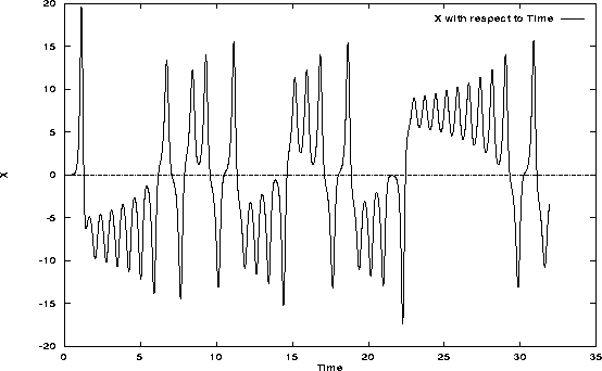
Figure 4.1: Lorenz Attractor X variable vs. Time
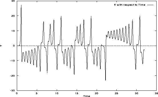
Figure 2.7: Lorenz Attractor Y variable vs. Time
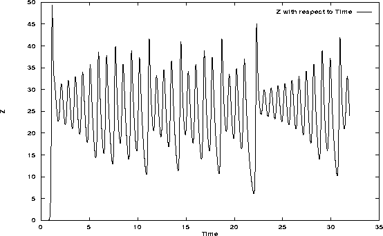
Figure 2.8: Lorenz Attractor Z variable vs. Time
As stated previously, the combination of all three variables locate a point in three dimensional space. The most common view of these three variables takes place in what mathematicians have come to refer to as phase space - a three dimensional plot of the system over all time. The thinking behind the phase space plot is to provide an idea of what the system is like by containing the output for a long period of time in a single graph. Viewed from the side, the phase space plot of this system is the following (Figure 2.9):
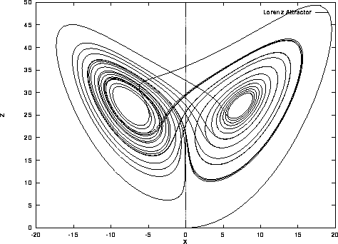
Figure 2.9: The Lorenz Attractor from the X-Z plane
Figure 2.9 is the combination of the x, y and z variables acting together over a period of thirty two ``seconds'' in my simulation. Every point from each calculation is drawn and left behind on the diagram to produce a time record. The image is best known as the ``Lorenz Attractor'' and is one of the earliest example of chaos ever recorded. It has also been referred to as ``Lorenz's Butterfly'' in honor of the butterfly effect. The Lorenz attractor always has the familiar butterfly shape, no matter how ``random'' each variable may appear to be on its own, the combination of the three always produces the same picture.
Figure 2.10 is another run of the Lorenz attractor program for slightly different initial conditions. Notice in figure 2.11, where it is plotted against the earlier x variable run, how the outputs stay nearly the same for a good portion of time at the beginning, but diverge into completely different patterns.
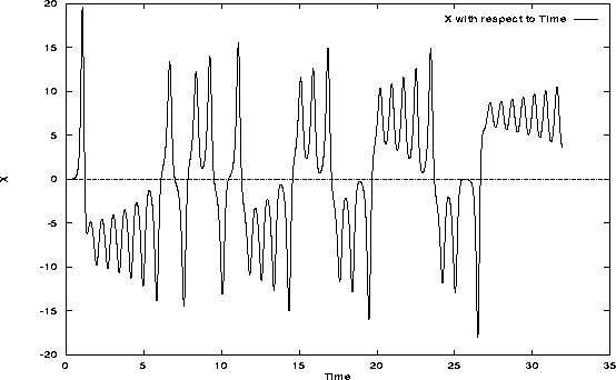
Figure 2.10: Lorenz Attractor X vs. Time for slightly different initial conditions
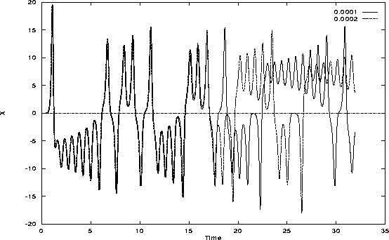
Figure 2.11: Lorenz Attractor X vs. Time comparison
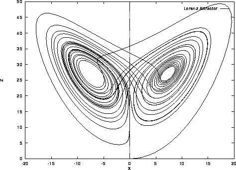
Figure 2.12: The Lorenz Attractor with slightly different initial conditions
I have reproduced again in figure 2.12 the Lorenz attractor, except this time with the same slight variation in initial conditions as observed in figures 2.10 and 2.11. It manages to maintain its same butterfly shape, despite the utter lack of correlation in figure 2.11. At first glance, there is what appears to be random fluctuations coming from what should be a completely deterministic set of equations - behavior completely unheard of. Behavior often discarded as simply an error in calculation. Lorenz was the first to recognize this erratic behavior as something other than error, and that everyone had been trying to view the world through a microscope. When he put the microscope aside and looked with his own eyes, what he saw was an undeniable order, born out of the randomness.
That's the beauty and underlying order in chaos. A system that is completely free willed when viewed from a certain perspective just happens to fall within a completely deterministic, predictable pattern.
Stochastic behavior occurring in a deterministic system is beginning to sound like a definition of life.